Understand the granular segregation and the transport equation

• [1] General Model For Segregation Forces in Flowing Granular Mixtures
• [2] Diffusion, mixing, and segregation in confined granular flows
• [3] On Mixing and Segregation: From Fluids and Maps to Granular Solids and Advection–Diffusion Systems

Introduction

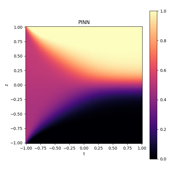
In this project, a PINN is trained to solve a 2D advection-segregation-diffusion problem.

\[\frac{\partial c_i}{\partial t} +\frac{\partial (w_{i}c_i)}{\partial z}=\frac{\partial}{\partial z} \Big( D\frac{\partial c_i}{\partial z} \Big),\]

with the following boundary conditions: \(\begin{cases} c_i(t=0, z) = 0.5 \\ w_{i}c_i|_{(t, z=0)}-D\frac{\partial c_i}{\partial z} |_{(t, z=H)} =0\\ w_{i}c_i|_{(t, z=0)}-D\frac{\partial c_i}{\partial z} |_{(t, z=H)}=0\\ \end{cases}\)
The objective is to predict the transient concentration profile:

Simplified Advection-Diffusion-Segregation

Sample the domain with data points and build a Neural Network to minimize the loss function:

\[Loss_{domain}=\frac{\partial c_i}{\partial t} +\frac{\partial (w_{i}c_i)}{\partial z} -\frac{\partial}{\partial z} \Big( D\frac{\partial c_i}{\partial z} \Big),\]

Loss function for boundary data points:

\[Loss_{BC}=(w_{i}c_i) - D\frac{\partial c_i}{\partial z}.\]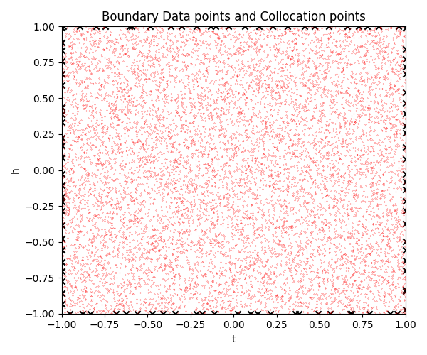

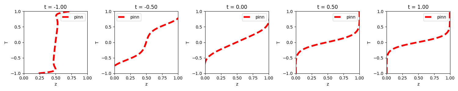
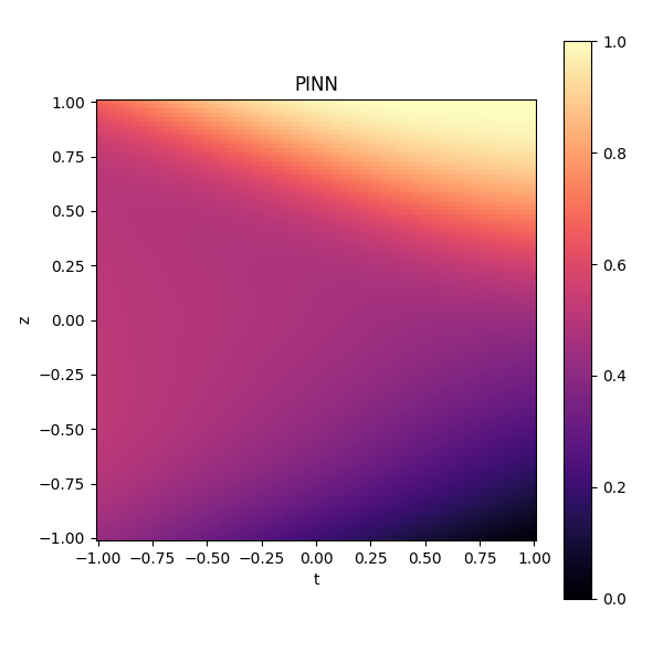
Linear Segregation

Assuming linear segregation velocity (Fan et al. 2014) and constant diffusion coefficient. \(\begin{cases} w_i=A\dot\gamma(1-c_i)\\ D=0.042\dot\gamma d^2\\ \end{cases}\)

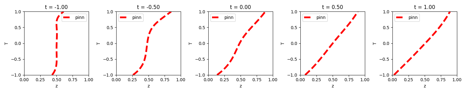
Large particle concentration profiles:

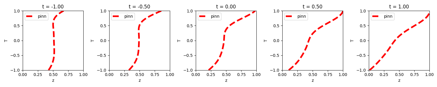
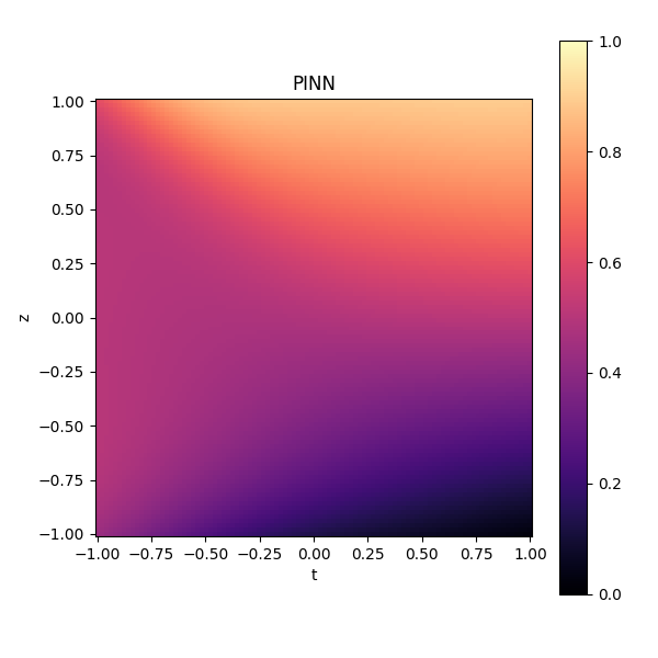
Pressure-corrected Linear Segregation

Assuming linear segregation velocity (Fan et al. 2014) and constant diffusion coefficient. \(\begin{equation} \begin{cases} w_i=A\dot\gamma(1-c_i) \sqrt{\frac{P_0}{P}}\\ D=0.042\dot\gamma d^2\\ \end{cases} \end{equation}\)

Large particle concentration profiles:

Pressure-corrected Linear Segregation + concentration dependent diffusion coefficient

Assuming linear segregation velocity (Fan et al. 2014) and constant diffusion coefficient. \(\begin{equation} \begin{cases} w_i=A\dot\gamma(1-c_i) \sqrt{\frac{P_0}{P}}\\ D=0.042\dot\gamma (\sum c_id_i)^2\\ \end{cases} \end{equation}\)

Large particle concentration profiles:

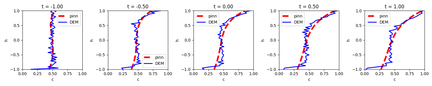
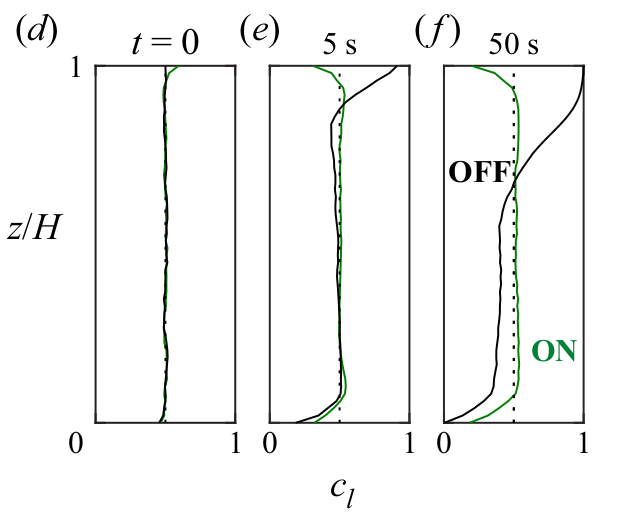
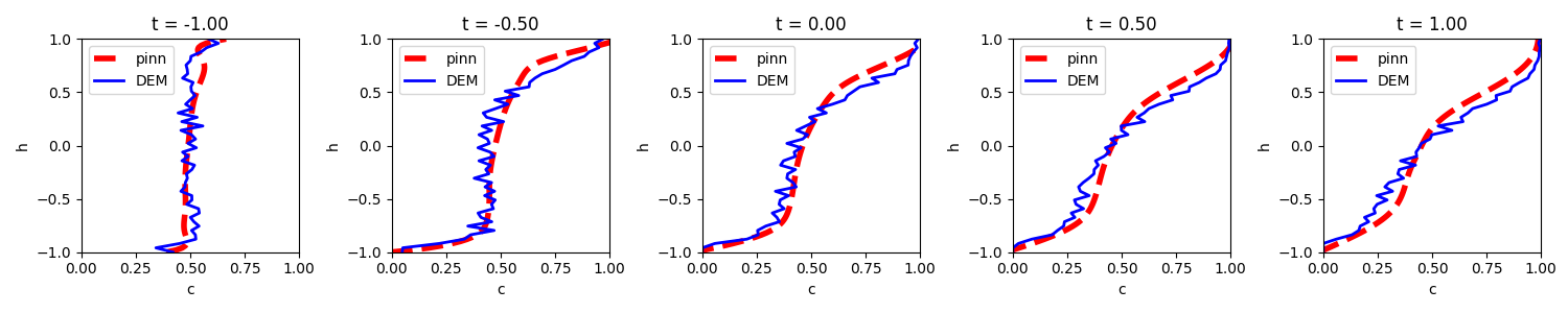
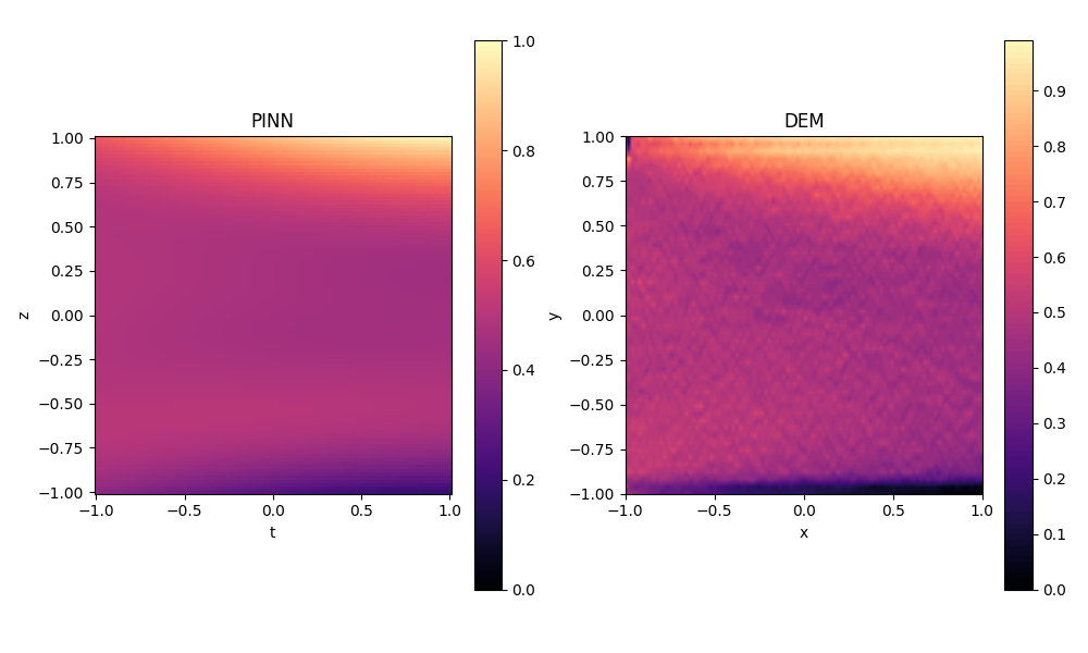
DEM-informed NN

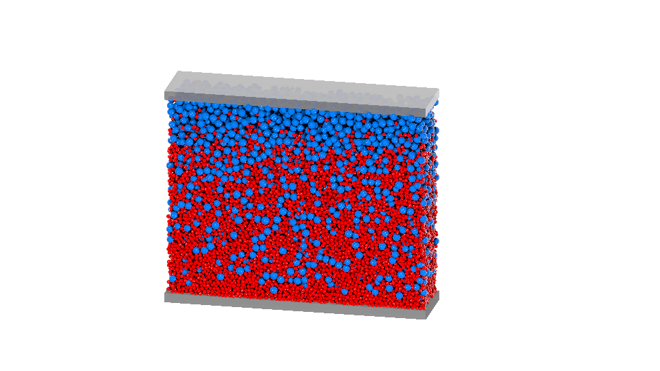
DEM simulations (\(R_d=2,~R_\rho=1,~t=37\,s\)):

Segregation flux is formed with unkown variables to identify: \(\begin{equation} \begin{cases} w_i=F_{x1} \tanh(F_{x2} \frac{c_s}{c_l})/C_d\eta\\ \Phi=F_{x3}(w_i-0.042\dot\gamma (\sum c_id_i)^2 \frac{\partial c_l}{\partial z})\\ \end{cases} \end{equation}\)

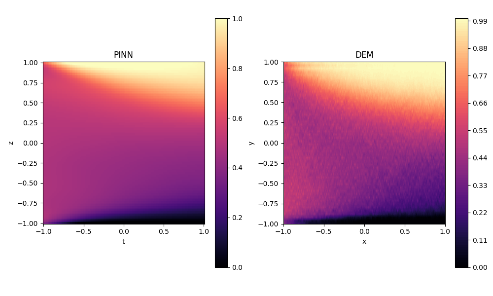
The variables are identified as: \(\begin{equation} \begin{cases} F_{x1}=2.1619\\ F_{x2}=1.3354\\ F_{x3}=2.4698\\ \end{cases} \end{equation}\)
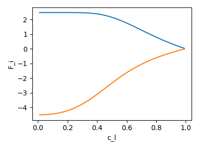
This implies a concentration dependence of force:

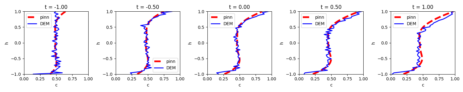
DEM-informed NN - reduce sample size

DEM simulations (\(R_d=2,~R_\rho=1,~t=10\,s\)):

The variables are identified as: \(\begin{equation} \begin{cases} F_{x1}=2.4664\\ F_{x2}=1.1263\\ F_{x3}=2.8693\\ \end{cases} \end{equation}\)

Does cubic segregation velocity model works better?

\[\begin{equation} \begin{cases} w_i=F_{x1} c_l+ F_{x2}c_l^2+F_{x3}c_l^3\\ \Phi=F_{x4}(w_i-0.042\dot\gamma (\sum c_id_i)^2 \frac{\partial c_l}{\partial z})\\ \end{cases} \end{equation}\]

Cubic segregation velocity model cannot capture the DEM profiles.