Physics Informed Neural Network
Overview
Links to run the code
Understand the granular segregation and the transport equation
- [1] General Model For Segregation Forces in Flowing Granular Mixtures
- [2] Diffusion, mixing, and segregation in confined granular flows
- [3] On Mixing and Segregation: From Fluids and Maps to Granular Solids and Advection–Diffusion Systems
PINN implementation
- https://github.com/nanditadoloi/PINN
- https://github.com/omniscientoctopus/Physics-Informed-Neural-Networks
- https://github.com/maziarraissi/PINNs
Here is a li
1. Introduction
An advection-diffusion transport equation has been successfully used to model the segregation. Within this continuum framework, the concentration of species \(i\) can be expressed as
\[\frac{\partial c_i}{\partial t} + {\nabla \cdot (\pmb u c_i)}={\nabla \cdot (D\nabla c_i)}.\]With assumption of incompressible flow and negligible vertical acceleration, the above equation in the \(z\) direction can be written as
\[\frac{\partial c_i}{\partial t} +\frac{\partial (w+w_{i})c_i}{\partial z}=\frac{\partial}{\partial z} \Big( D\frac{\partial c_i}{\partial z} \Big),\]or, rearranging, as
\[w_{i}c_i-D\frac{\partial c_i}{\partial z}=0,\]where \(w_{i}\) is the segregation velocity relative to the bulk velocity \(w\).
| full model | simplified model | ||
|---|---|---|---|
| intruder scaled segregation force | \(F_{i,0}\) | \(-f^g(R)\frac{\partial{p}}{\partial{z}}V_i+f^k(R)\frac{p}{\dot\gamma}\frac{\partial\dot\gamma}{\partial{z}}V_i\) | |
| Mixture scaled segregation force | \(\hat F_{l}\) \(\hat{F}_{s}\) | \((\hat{F}_{l,0}-\cos{\theta})\textrm{tanh}\Big( \frac{\cos{\theta}-\hat{F}_{s,0}}{\hat{F}_{l,0}-\cos{\theta}}\frac{c_s}{c_l} \Big)\) \(-(\hat{F}_{l,0}-\cos{\theta}){\frac{c_l}{c_s}}\textrm{tanh}\Big( \frac{\cos{\theta}-\hat{F}_{s,0}}{\hat{F}_{l,0}-\cos{\theta}}\frac{c_s}{c_l} \Big)\) | |
| effective friction | \(\mu_{eff}\) | \(\mu_s+\frac{\mu_2-\mu_s}{I_c/I+1}\) | |
| viscosity | \(\eta\) | \(\mu_{eff} \frac{P}{\dot\gamma}\) | |
| drag coefficient | \(c_{d,l}\) \(c_{d,s}\) | \([k_1-k_2\exp(-k_3 R)]+s_1 I R +s_2 I (R_\rho-1)\) \(c_{d,l}/R^2\) | |
| segregation velocity | \(w_l\) \(w_s\) | \(\frac{ \hat F_{l} m_l g_0}{c_{d,l} \pi \eta d_l}\) \(-\frac{ \hat F_s m_s g_0}{c_{d,s} \pi \eta d_s}\) | \(0.26 d_s \ln R \dot\gamma (1-c_i)\) |
| diffusion coefficient | \(D\) | \(0.042 \dot \gamma (c_ld_l+c_sd_s)^2\) | \(0.042 \dot \gamma {\bar d}^2\) |
2. Physics Informed Neural Network
import math
import numpy as np
import torch
import torch.nn as nn
device = (
    "cuda"
    if torch.cuda.is_available()
    else "mps"
    if torch.backends.mps.is_available()
    else "cpu"
)

class Net(nn.Module):
    def __init__(self):

        # 6 layer neural network
        super(Net, self).__init__()
        self.ln1 = nn.LayerNorm(100)
        self.ln2 = nn.LayerNorm(100)
        self.ln3 = nn.LayerNorm(100)
        self.ln4 = nn.LayerNorm(100)

        self.hidden_layer1 = nn.Linear(1,100)
        self.hidden_layer2 = nn.Linear(100,100)
        self.hidden_layer3 = nn.Linear(100,100)
        self.hidden_layer4 = nn.Linear(100,100)
        self.hidden_layer5 = nn.Linear(100,100)
        self.output_layer = nn.Linear(100,1)
        self.mse=torch.nn.MSELoss()

        # particle properties in S.I unit
        self.rd=2
        self.dl=0.004
        self.rho=1000
        self.c_diffusion=0.042
        self.ds=self.dl/self.rd
        self.rds=1/self.rd
        self.ml=4/3*math.pi*0.002**3*self.rho
        self.ms=4/3*math.pi*0.001**3*self.rho


        # flow configuration (uniform shear)
        self.gamma=100
        self.phi=0.55
        self.g=9.81
        self.h0=0.01
        self.p0=self.h0*self.rho*self.g*self.phi

        # segregation force calculation
        self.theta=torch.tensor(np.cos(0), dtype=torch.float32, requires_grad=True).to(device)
        #  Duan et al. 2024
        _intruder_l=(1-1.43*np.exp(-self.rd/0.92))*(1+3.55*np.exp(-self.rd/2.94))*self.phi
        _intruder_s=(1-1.43*np.exp(-self.rds/0.92))*(1+3.55*np.exp(-self.rds/2.94))*self.phi

        self.intruder_l=torch.tensor(_intruder_l, dtype=torch.float32, requires_grad=True).to(device)
        self.intruder_s=torch.tensor(_intruder_s, dtype=torch.float32, requires_grad=True).to(device)

    def forward(self, z):
        # if time dimensino is considered, concatenated first, i.e. torch.cat([z,t],axis=1)
        layer1_out = self.ln1(torch.sigmoid(self.hidden_layer1(z)))
        layer2_out = self.ln2(torch.sigmoid(self.hidden_layer2(layer1_out)))
        layer3_out = self.ln3(torch.sigmoid(self.hidden_layer3(layer2_out)))
        layer4_out = self.ln4(torch.sigmoid(self.hidden_layer4(layer3_out)))
        layer5_out = torch.sigmoid(self.hidden_layer5(layer4_out))
        output = self.output_layer(layer5_out) ## For regression, no activation is used in output layer
        return output

    def loss(self):


        # PDE loss
        z_collocation = np.random.uniform(low=0.0, high=0.1, size=(10001,1))

        z = torch.tensor(z_collocation, dtype=torch.float32, requires_grad=True).to(device)

        c = self(z)

        p=self.rho*self.phi*self.g*z+self.p0
        inert=self.gamma*(c*0.004+(1-c)*(0.004/self.rd))/torch.sqrt(p/self.rho);
        mu_eff=0.364+(0.772-0.364)/(0.434/inert+1)
        eta=mu_eff*p/self.gamma

        mixture_l=(self.intruder_l-self.theta)*torch.tanh((self.theta-self.intruder_s)/(self.intruder_l-self.theta)*self.ml/self.ms*(1-c)/c)
        mixture_s=-(self.intruder_l-self.theta)*c/(1-c)*self.ms/self.ml*torch.tanh((self.theta-self.intruder_s)/(self.intruder_l-self.theta)*self.ml/self.ms*(1-c)/c)


        cd=(2-7*math.exp(-2.6*self.rd))+0.57*inert*self.rd

        wseg=mixture_l*self.ml*self.g / (cd*math.pi*eta*0.004)

        c_z = torch.autograd.grad(c.sum(), z, create_graph=True)[0]

        # Duan et al. 2024
        pde=(wseg*c-0.042*self.gamma*torch.square((1-c)*self.ds+c*self.dl)*c_z)*100

        # Schlick et al. 2015
        # simplified with constant diffusion coefficient
        # pde = (1/0.1 *(1-c)*c - c_z )*10

        target = torch.zeros_like(pde,requires_grad=False)
        pde_loss=self.mse(pde,target)


        # Mass conservation loss
        x_bc = torch.linspace(0, 0.1, 10001,requires_grad=True).to(device)
        x_bc = x_bc.unsqueeze(-1)
        u_bc = self(x_bc)
        u_bc=torch.mean(u_bc)

        target=torch.zeros_like(u_bc,requires_grad=False).to(device)+0.5
        mass_loss=self.mse(u_bc,target)

        return mass_loss  + pde_loss
3. Train
net = Net()
net = net.to(device)
mse_cost_function = torch.nn.MSELoss() # Mean squared error
optimizer = torch.optim.Adam(net.parameters(),lr=0.002)


iterations = 5000
previous_validation_loss = 99999999.0
for epoch in range(iterations):
    optimizer.zero_grad() # to make the gradients zero
    loss=net.loss()
    loss.backward() # This is for computing gradients using backward propagation
    optimizer.step() # This is equivalent to : theta_new = theta_old - alpha * derivative of J w.r.t theta
    if loss.data<1e-6:
        break
    with torch.autograd.no_grad():
    	print(epoch,"Traning Loss:",loss.data)
4. Results
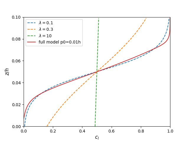
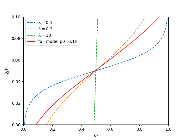
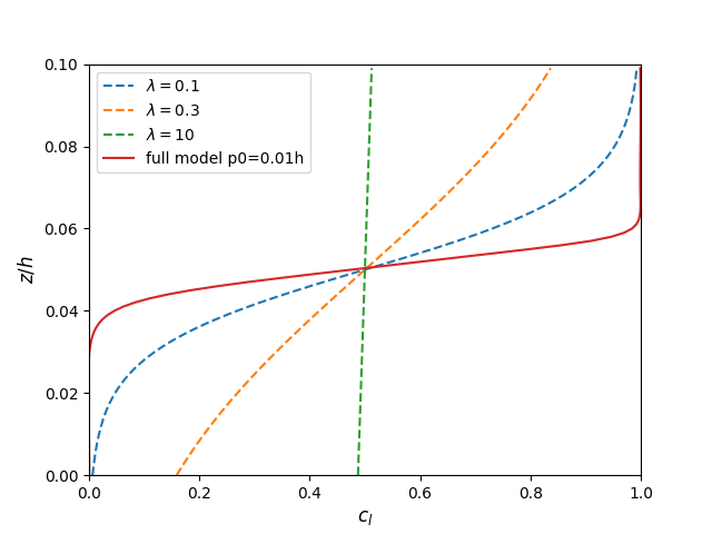
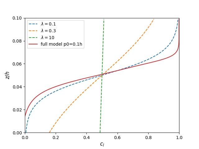
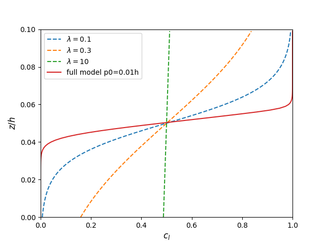
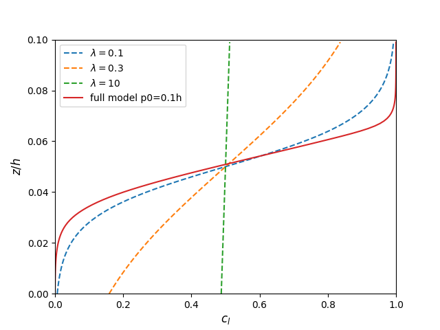
The full model prediction is compared to the previous model by Schlick et al. 2015 with different values of \(\lambda\).
\[\frac{d_c}{d_z}=\frac{1}{\lambda}c_l(1-c_l)\]4.1 Uniform shear
4.2 Exponential shear
5. Improvements
- Add loss function for \(c\) out of range 0 to 1
- Add a learning rate scheduler to reduce learning rate at loss plateau (lr reduced from 1e-3 to 1e-5)
After these changes, the overall loss is reduced to 1e-8
5.1 Exponential shear
Enjoy Reading This Article?
Here are some more articles you might like to read next: